4. EXPERIMENTAL PROCEDUR
4.2. Practice 2: Determination of the characteristic curve of the system
Objective
In this case, what we find is the characteristic curve of the installation.
we find the characteristic curve of the installation for the loss of pressure in the pipes in a given volume.
Introduction
In the scheme shown below, we see the movement of the fluid:
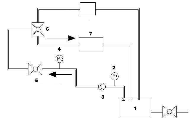
Where:
1) Water tank.
2) Manometer (P1).
3) Pump.
4) Manometer (P2).
5) Valve.
6) Spherical valve of three way.
7) Diaphragm.
From here you can find the operating point of the pump. We find the operating point of the bomb from the point it crosses the characteristic curve of the pump with the team.
Material
In this case we only need the pilot plant.
Procedure
To carry out this practice, you must follow these steps:
1. Observe the level water of the tank (1), is 10 cm from the surface.
2. Watch it is plugged.
3. Remove the emergency stop (a).
4. Put the device in position "ON" with the red wheel (b).
5. Before turning on the pump, check spherical valve of three way(6) is closed (position "OFF").
6. Press the Power button (c).
7. Opening the spherical valve of three way(ON).
8. With the wheel of potentiometer (f), put the equipment to 2400 rpm, you must do it gradually, not abruptly.
9. Open up the valve (5) which is under the manometer.
10. Connect two hoses the pressure sensor to diaphragm (7). If we not get any value in the screen flow, is that they are poorly connected, therefore exchanging the position.
11. Purge air (II) tubes opening the purge valve.
12. Note the angular velocity (g), flow (d) P1 and P2.
13. Modify at 2300 rpm with the wheel again and record your results.
14. Repeat the procedure decreasing 100 to 100 to arrive at a ω = 1200rpm.
15. Finished practice, put spherical valve of three way (6) in position "OFF
16. Stop the machine, with the stop button (c) the wheel and red (b).
17. Pressing the emergency stop (a).
Then, using the video, we can see how it performs in practice:
Expression of result
You must fill out the following table and make the necessary calculations that are summarized in the section on basics:
ω (rpm) |
P1 (bar) |
P2 (bar) |
G (m3/h) |
u1(m/s) |
u2(m/s) |
H (m) |
2400 |
|
|
|
|
|
|
2300 |
|
|
|
|
|
|
2200 |
|
|
|
|
|
|
2100 |
|
|
|
|
|
|
2000 |
|
|
|
|
|
|
1900 |
|
|
|
|
|
|
1800 |
|
|
|
|
|
|
1700 |
|
|
|
|
|
|
1600 |
|
|
|
|
|
|
1500 |
|
|
|
|
|
|
1400 |
|
|
|
|
|
|
1300 |
|
|
|
|
|
|
1200 |
|
|
|
|
|
|
If you represent the height (H) in the axis of abscises and volumetric flow (G) in the axis of the order, we obtain the following graph:

We can observe the trend that follows the curve is rising, as we increase the flow, so does the height.
As mentioned in the previous section, the height is related to the pressure difference using the formula:

Therefore, as the pressure difference between P1 and P2 decreases, the height increases.
Once we've already found the characteristic curve of the pump and the system we can find the operating point of the team.
This is the point where the heights of the two curves coincide, as shown in the figure:

This is the point where our team will work under the best conditions and performance.